Flink SQL DML
Updates
Created 10/24 Revised 4/07/26 Add new examples 06/15/2026
This chapter continues the discussion of best practices for implementing Flink SQL Data Manipulation Language (DML) queries. DML defines statements that modify data without changing metadata.
Sources of information
- Confluent SQL documentation for DML samples
- Apache Flink SQL
- Confluent Developer Flink tutorials
- The Flink built-in system functions.
Common Patterns
It is important to recall that a SELECT applies to a stream of records, so the results change as new records arrive. The query below shows the latest top 10 orders; when a new record arrives, the list updates.
What are the different SQL execution modes? (OSS)
Using the previous table, you can count rows with:
and we get different behavior depending on the execution mode:
set 'execution.runtime-mode' = 'batch';
# default one
set 'execution.runtime-mode' = 'streaming';

set 'sql-client.execution.result-mode' = 'table';
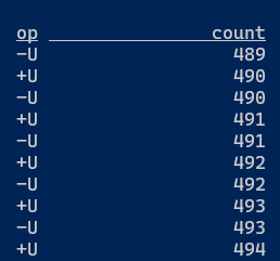
In changelog mode, the SQL Client doesn't just update the count in place, but instead displays each message in the stream of updates it's receiving from the Flink SQL runtime.
See this lab in changelog mode and this section in SQL concepts chapter.
Playing with Inserts
- Add a NULL to a string column:
insert into sl_raw_groups values('grp_001','tenant-01','gp_n1', 'g_typ_1', CAST(NULL AS STRING), false) - Specifying the columns to use:
insert into sl_raw_groups(group_id,tenant_id) VALUES('grp_001','tenant-01'), this will populate the missing columns with null.
Filtering
- Start with this Confluent tutorial or the Apache Flink
SELECTdocumentation. SELECT ... FROM ... WHERE ...uses column projections or filters and is stateless. Unless the output table has aretractchangelog while the input isupsert, the sink will use achangelog materializer(see section below).SELECT DISTINCTremoves duplicate rows, which requires keeping state for each distinct row.
How to filter out records?
using the WHERE clause
Count the number of events related to a cancelled flight (need to use one of the selected field as grouping key):
select flight_id, count(*) as cancelled_fl from FlightEvents where status = 'cancelled' group by flight_id;
Recall that this query produces a dynamic table.
HAVING to filter after aggregation
The HAVING clause is used to filter results after the aggregation (i.e., like GROUP BY). It is similar to the WHERE clause, but while WHERE filters rows before aggregation, HAVING filters rows after aggregation.
How to combine records from multiple tables (UNION)?
When the two tables have the same number of columns of compatible types, we can combine them:
See product documentation on UNION. Remember that UNION applies DISTINCT and removes duplicates, while UNION ALL keeps all rows, including duplicates.
How to filter rows whose column content does not match a regular expression?
Use REGEX
Navigate a hierarchical structure in a table
The table uses a node-and-ancestors representation. Suppose the graph represents a procedure at the highest level, then an operation, then a phase, and a phase step at level 4. The procedures table can have rows like:
id, parent_ids, depth, information
'id_1', [], 0 , 'procedure 1'
'id_2', ['id_1'], 1 , 'operation 1'
'id_3', ['id_1','id_2'], 2 , 'phase 1'
'id_4', ['id_1','id_2','id_3'], 3 , 'phase_step 1'
'id_5', ['id_1','id_2','id_3'], 3 , 'phase_step 2'
Suppose we want to extract matching procedure_id, operation_id, phase_id, and phase_step_id like:
id, procedure_id, operation_id, phase_id, phase_step_id, information
'id_1', 'id_1', NULL, NULL, NULL, 'procedure 1'
'id_2', 'id_1', 'id_2', NULL, NULL, 'operation 1'
'id_3', 'id_1', 'id_2', 'id_3', NULL, 'phase 1'
'id_4', 'id_1', 'id_2', 'id_3', 'id_4', 'phase_step 1'
'id_5', 'id_1', 'id_2', 'id_3', 'id_5', 'phase_step 2'
if the depth is 3, then the response should have all ids populated, if 0 only the top level is returned.
with `procedures` as (
    select 'id_1' as id, array[''] as parentIds, 0 as `depth` , 'procedure 1' as info
    UNION ALL
    select 'id_2' as id, array['id_1'] as parentIds, 1 as `depth` , 'operation 1' as info
    UNION ALL
    select 'id_3' as id, array['id_1','id_2'] as parentIds, 2 as `depth`, 'phase 1' as info
    UNION ALL
    select 'id_4' as id, array['id_1','id_2','id_3'] as parentIds, 3 as `depth`, 'phase_step 1' as info
    UNION ALL
    select 'id_5' as id, array['id_1','id_2','id_3'] as parentIds, 3 as `depth`, 'phase_step 2' as info
    )
select
    id,
    parent_id,
    case when `depth` = 3 then id end as phase_step_id,
    case when `depth` = 2 then id end as phase_id,
    case when `depth` = 1 then id end as operation_id,
    case when `depth` = 0 then id end as procedure_id,
    info from `procedures` cross join unnest(parentIds) as ids(parent_id)
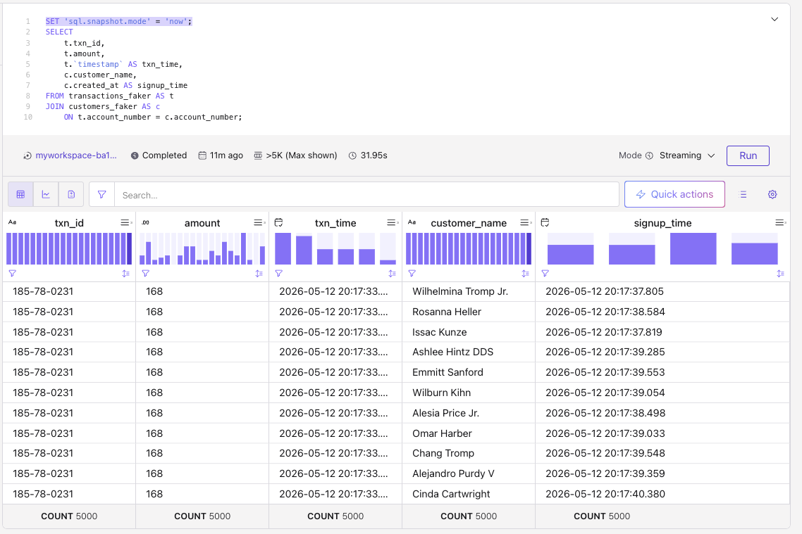
Snapshot queries
Enabling snapshot query forces Flink to process data in a topic as a bounded set, from the earliest available record to the latest offset when the query is submitted. On Confluent cloud, when Tableflow is enabled on the topic, the query will also read the historical data from the Iceberg table and then read only the latest records from the Kafka topic.
It is used for reporting, assessing historical data, investigating issues on past data.
When summitting statement via the REST API, the mode is set via spec properties.
Flink automatically switches to batch mode processing. Snapshot queries use read-committed as the default isolation level, which aligns with Kafka’s exactly-once semantics (EOS).
Deduplication
Deduplication will occur on upsert table with primary key: the last records per $rowtime or other timestamp will be kept. When the source table is in append mode, the approach is to use the ROW_NUMBER() combined with OVER():
CREATE TABLE unique_clicks
AS SELECT ip_address, url, TO_TIMESTAMP(FROM_UNIXTIME(click_ts_raw)) as click_timestamp
    FROM (
        SELECT *,
        ROW_NUMBER() OVER ( PARTITION BY ip_address ORDER BY TO_TIMESTAMP(FROM_UNIXTIME(click_ts_raw)) ASC) as rownum
        FROM clicks
        )
    WHERE rownum = 1;
- The query is designed to identify and persist only the earliest record. Once the record is written to the table_deduped any subsequent events pertaining to the same
ip_addressare effectively discarded by theWHERE rownum = 1filter. ROW_NUMBER()assigns a unique, sequential number to each row. It is part of the Top-N query pattern.- Use
OVERaggregation to compute aggregate values for each input row under a window specification and a filter condition to express a Top-N query. Combined withPARTITION BY, Flink supports per-group Top-N. - The inner query adds a
row_numfor each row in each partition. - The subsequent
WHERE rownum = 1clause filters the results to retain only the very first event observed for each uniqueip_addressbased on its timestamp. - The created table is an append table. There is no mechanism within this query to generate update or delete operations for records that have already been processed. Even if the underlying
clickstable has a primary key defined, the transformation applied here dictates that theunique_clickstable will only ever grow by appending new, uniqueip_addressentries. - If the sort order is
DESC, when a new record arrives a retraction or update may be emitted. - After deduplication, the upsert sink primary key should align with the partition keys used in the deduplication logic.
See this example in the Confluent product documentation: select * from dedup_table; returns eight messages with no duplicates, and the Kafka topic also contains eight messages.
That walkthrough does not show that the last message per key is kept. The deduplication sample shows how an upsert table removes duplicates and retains the last record per key.
- Confluent Cloud has limitations:
ORDER BYin this pattern may be restricted to a timestamp column in ascending order. - Example of deduplication on OSS Flink where
ORDER BYcan use columns of other types (where supported).
Transformation
Some important resources:
- Transform a Topic with Confluent Cloud for Apache Flink (product doc) covers topic transformation from the Data Portal: Actions → Transform Topic, which creates a CTAS Flink SQL statement and deploys it to the configured compute pool. This is efficient for Avro-to-JSON conversion, field renames, and primary-key changes.
How to transform a field representing epoch to a timestamp?
epoch is a BIGINT.
How to change a date string to a timestamp?
See all the date and time functions.
Use the kafka timestamp for a null timestamp
If created_date is NULL then use the $rowtime.
How to compare a date field with current system time?
If the target table uses changelog-mode = upsert, using now() is problematic because the execution time is not deterministic per row. The statement above is appropriate mainly for append mode.
How to extract the number of days between a date field and now?
The difference is in timestamp types. First cast the DATE column to a timestamp, then use CURRENT_DATE and the DAY unit. See supported units (SECOND, MINUTE, HOUR, DAY, MONTH, or YEAR).
How to access elements of an array of rows?
The table has a column that is an array of rows.
To create one record per row within the array, so exploding the array, use CROSS JOIN UNNEST:
 SELECT
    t.key_col,
    unnested_row.id,
    unnested_row.name
FROM
    my_table AS t
CROSS JOIN UNNEST(t.nested_data) AS unnested_row;
Each row in the nested_data array will be a row in the output table with the matching key_col.
How to use conditional functions?
Flink has built-in conditional functions (see also Confluent), especially CASE WHEN:
How to mask a field?
Create a new table from the existing one, and then use REGEXP_REPLACE to mask an existing attribute
JSON Transformation
Flink provides JSON built-in functions to extract information from json string. '$' denotes the root node in a JSON path.
Paths can access properties (\(.a), array elements (\).a[0].b), or branch over all elements in an array ($.a[*].b).
There are really two groups of function: extracting value from a JSON string:
- Return scalar value with JSON_VALUE
-
Return a string or array of strings- lax is to suppress errors and returns NULL or empty results if the path does not match the JSON schema.
-
Build JSON_OBJECT as string from a list of key-value pairs,
Suppose that data is a <ROW<
versionDOUBLE,transactionIdVARCHAR(2147483647)>>. To create a json object as a string like '{"version": 1.1}'
How to access JSON data from a string column that contains a JSON object?
Use json_query function in the select.
Use json_value() when you need a scalar extracted from JSON object content.
How to transform a JSON array column (named data) into an array and then generate n rows?
Returning an array from a json string:
To create as many rows as there are elements in the nested array:
SELECT existing_column, anewcolumn from table_name
cross join unnest (json_query(`data`, '$' RETURNING ARRAY<STRING>)) as t(anewcolumn)
UNNEST returns a new row for each element in the array See multiset expansion doc
Extract content from a JSON array as strings and explode to multiple rows?
The input record has a parameters column with an array of objects (key-value fields), like:
[{"parameter_name": "Pressure", "parameter_value": 10.0, "parameter_type": "float", "parameter_tolerance": 1.0}, {"parameter_name": "FlowRate", "parameter_value": 2.5, "parameter_type": "float", "parameter_tolerance": 0.5}, {"parameter_name": "MotorSpeed", "parameter_value": 3200.0, "parameter_type": "float", "parameter_tolerance": 150.0}]
CROSS JOIN UNNEST on an array. Then extract each JSON object. Guard with conditions on the parameters string so JSON_QUERY receives valid input. SELECT
prescription_id,
patient_id,
device_id,
medication_or_therapy,
JSON_VALUE(param_obj, 'lax $.parameter_name') AS metric_name,
CAST(JSON_VALUE(param_obj, 'lax $.parameter_value' RETURNING DOUBLE) AS DOUBLE) AS target_value,
CAST(JSON_VALUE(param_obj, 'lax $.parameter_tolerance' RETURNING DOUBLE) AS DOUBLE) AS tolerance_range,
start_date,
end_date
FROM `healthcare.public.prescriptions`
CROSS JOIN UNNEST(
JSON_QUERY(parameters, 'lax $[*]' RETURNING ARRAY<STRING>)
) AS t(param_obj)
WHERE parameters IS NOT NULL AND TRIM(parameters) <> '' AND TRIM(parameters) <> '[]';
How to implement the equivalent of SQL explode?
In classical SQL, EXPLODE creates a row for each element in the array or map and ignores null or empty entries in the array.
SQL also defines EXPLODE_OUTER, which returns all values in the array, including null or empty entries.
To translate this to Flink SQL you can use MAP_ENTRIES and MAP_FROM_ARRAYS. MAP_ENTRIES returns an array of all entries in the given map. MAP_FROM_ARRAYS returns a map created from parallel arrays of keys and values.
As presented in previous question, CROSS JOIN UNNEST(array) is also the recommended solution.
Statement Set
Bundling statements in a single set reduces repeated reads from the source for each INSERT: one read from the source is executed and shared across downstream inserts.
Do not use a statement set when the sources differ for each statement inside the set. If one statement in the set fails, all queries in the set fail. State is shared across statements in the set, so one stateful query can affect the others.
How to route late messages to a DLQ using a statement set?
First, create a DLQ table like late_orders based on the order table:
Group the main stream processing and late-arrival handling in one statement set:
EXECUTE STATEMENT SET
BEGIN
    INSERT INTO late_orders SELECT * FROM orders WHERE `$rowtime` < CURRENT_WATERMARK(`$rowtime`);
    INSERT INTO order_counts -- the sink table
        SELECT window_time, COUNT(*) as cnt
        FROM TABLE(TUMBLE(TABLE orders DESCRIPTOR(`$rowtime`), INTERVAL '1' MINUTE))
        GROUP BY window_start, window_end, window_time
END
Stateful aggregations
An aggregate function computes a single result from multiple input rows.
GROUP BY
Classical SQL grouping of records, but with streaming the state may grow without bound. The size depends on the number of groups and how much data must be retained per group. group by generates upsert events as it manages key-value and repartitions data.
EXPLAIN
SELECT
  account_number,
  transaction_type,
  SUM(amount)
  FROM `transactions`
  where transaction_type = 'withdrawal'
  GROUP BY account_number,  transaction_type
HAVING SUM(amount) > 5000
The physical plan looks like
== Physical Plan ==

StreamSink [6]
  +- StreamCalc [5]
    +- StreamGroupAggregate [4]
      +- StreamExchange [3]
        +- StreamCalc [2]
          +- StreamTableSourceScan [1]

== Physical Details ==

[1] StreamTableSourceScan
Table: `j9r-env`.`j9r-kafka`.`transactions`
Primary key: (txn_id)
Changelog mode: append
Upsert key: (txn_id)
State size: low
Startup mode: earliest-offset
Key format: avro-registry
Key registry schemas: (:.:transactions/100220)
Value format: avro-registry
Value registry schemas: (:.:transactions/100219)

[4] StreamGroupAggregate
Changelog mode: retract
Upsert key: (account_number,transaction_type)
State size: medium
State TTL: never

[5] StreamCalc
Changelog mode: retract
Upsert key: (account_number,transaction_type)

[6] StreamSink
Table: Foreground
Changelog mode: retract
Upsert key: (account_number,transaction_type)
State size: low
DISTINCT
Remove duplicates before aggregating:
ARRAY_AGG
Array aggregation combines multiple data elements into a single array. It is widely used to regroup data points for downstream processing.
This Flink ARRAY_AGG aggregate function is common in record transformations. It returns an array whose elements come from multiple input rows.
Start with simple array indexing (indexes are 1-based through n). Below, VALUES creates in-memory test data in table alias T with column array_field:
The following SQL creates a view with an array aggregate: it collects URLs per user_id over one-minute tumbling windows.
CREATE VIEW visited_pages_per_minute AS
SELECT
    window_time,
    user_id,
    ARRAY_AGG(url) AS urls
FROM TABLE(TUMBLE(TABLE `examples.marketplace.clicks`, DESCRIPTOR(`$rowtime`), INTERVAL '1' MINUTE))
GROUP BY window_start, window_end, window_time, user_id;
-- once the view is created
SELECT * from visited_pages_per_minute;

-- it is possible to expand an array into multiple rows using cross join unnest

SELECT v.window_time, v.user_id, u.url FROM visited_pages_per_minute AS v
CROSS JOIN UNNEST(v.urls) AS u(url)
Important: new clicks for the same user_id with a new URL produce a new output row with the updated aggregated array. See cc-array-agg study.
To optimize processing, deduplicate and/or filter before aggregating; a Flink view is a typical pattern:
create view suites_versioned as
select  suite_id, suite_name, asset_id, asset_name, asset_price_min, asset_price_max, ts_ltz
from (
    select *,
       ROW_NUMBER() OVER (PARTITION BY suite_id, asset_id ORDER BY ts_ltz DESC) as rn
        from suites
    ) where rn = 1;
Then the array aggregation:
select
    suite_id,
    ARRAY_AGG(ROW (asset_id, asset_name,  ROW(asset_price_min, asset_price_max))) as asset_data,
    max(ts_ltz) as ts_ltz
from suites_versioned group by suite_id;
As in the example above, the array element type can be a row containing nested rows. See SQL examples.
OVER
OVER aggregations compute an aggregated value for every input row over a range of ordered rows. They do not reduce row count the way GROUP BY does; they emit one result per input row.
OVER specifies the time window over which the aggregation is performed. A classical example is to get a moving sum or average: the number of orders in the last 10 seconds:
SELECT
    order_id,
    customer_id,
    `$rowtime`,
    SUM(price) OVER w AS total_price_ten_secs,
    COUNT(*) OVER w AS total_orders_ten_secs
FROM `examples`.`marketplace`.`orders`
WINDOW w AS (
    PARTITION BY customer_id
    ORDER BY `$rowtime`
    RANGE BETWEEN INTERVAL '10' SECONDS PRECEDING AND CURRENT ROW
)
The window definition is externalized and can be used for multiple aggregates, like the SUM() and the COUNT() example, above.
The source topic should be in append mode because over-window aggregation does not support retraction/update semantics. OVER is useful when each input row must be evaluated against a time or row interval.
LAG and OVER
To detect when orders exceed limits for the first time and when aggregates later fall below other limits, use LAG.
-
Compute the total price and # of orders for a period of 10s for each customer
WITH orders_ten_secs AS ( SELECT order_id, customer_id, `$rowtime`, SUM(price) OVER w AS total_price_ten_secs, COUNT(*) OVER w AS total_orders_ten_secs FROM `examples`.`marketplace`.`orders` WINDOW w AS ( PARTITION BY customer_id ORDER BY `$rowtime` RANGE BETWEEN INTERVAL '10' SECONDS PRECEDING AND CURRENT ROW ) ), -
Get previous orders and current order per customer
-
Filter orders when the order price and number of orders were above some limits for previous or current order aggregates
SELECT customer_id, 'BLOCK' AS action, `$rowtime` AS updated_at
FROM orders_ten_secs_with_lag
WHERE
    (total_price_ten_secs > 300 AND total_price_ten_secs_lag <= 300) OR
    (total_orders_ten_secs > 5 AND total_orders_ten_secs_lag <= 5)
UNION ALL
SELECT customer_id, 'UNBLOCK' AS action, `$rowtime` AS updated_at
FROM orders_ten_secs_with_lag
WHERE
    (total_price_ten_secs <= 300 AND total_price_ten_secs_lag > 300) OR
    (total_orders_ten_secs <= 5 AND total_orders_ten_secs_lag > 5);
Aggregation over the last n preceding elements
The OVER window ends at the current row and stretches backward through the stream for a bounded interval, either in time or by row count. For example counting the number of flight_schedule events of the same key over the last 100 events:
select
    flight_id,
    evt_type,
    count(evt_type) OVER w as number_evt
from flight_events
window w as (partition by flight_id order by $rowtime rows between 100 preceding and current row);
The results are updated for every input row. The partition is by flight_id. Order by $rowtime is necessary.
When and how to use custom watermark?
Developers should define a custom watermark strategy when there are few records per topic or partition, a large watermark delay is required, or a non-default event-time column is used. The default uses SOURCE_WATERMARK(), a watermark supplied by the source. A common explicit choice is maximum-out-of-orderness so late-arriving events can still fall in the correct window, trading latency for accuracy. Example:
The minimum out-of-orderness is 50ms and can be set up to 7 days. See Confluent documentation.
Joins
When you run a join in a database, the result reflects the join state at execution time. In streaming, as both sides of a join receive new rows, both sides keep evolving. This is a continuous query on dynamic tables, and the engine must retain substantial state—effectively rows from each input.
Below is a common join we do between two tables:
SELECT t.amount, t.order_type, s.name, s.opening_value FROM transactions t
LEFT JOIN stocks s
ON t.stockid = s.id
On the left, the fact table changes at high velocity; events are typically append-only or immutable. On the right, the dimension table receives new records more slowly.
When doing a join, Flink needs to fully materialize both the right and left of the join tables in state, which may cost a lot of memory, because if a row in the left-hand table (LHT), also named the probe side, is updated, the operator needs to emit an updated match for all matching rows in the right-hand table (RHT) or build side. The cardinality of right side will be mostly bounded at a given point of time, but the left side may vary a lot. A join emits matching rows to downstream operator.
The key points to keep in mind are:
- Regular joins typically produce a full cross-product of all matching records. However, in streaming scenarios, this behavior is often undesirable, for example if you want to enrich an event with additional information, because the state to keep in distributed memory may become too big.
- When the RHS is an upsert table, the join output is often upsert-shaped as well: results may be re-emitted when the RHS changes. To pin dimension values to event time, use a temporal join so the RHS is as of the LHS event time (time-versioned enrichment).
- See basic joins examples
- Flink must handle the scenario where left-side events do not have corresponding right-side events at the time of processing. The Upsert table allows Flink to store unmatched left records and update them when matching right records arrive later, ensuring all left records are included in the result, thus supporting the LEFT JOIN semantics effectively in a streaming context
-
To avoid state growth, it is interesting to set time to live constraint (
/*+ STATE_TTL(o='2h', p='30d') */) on both tables like: -
Join order matters: prefer joining the slowest-changing dimension first when you can.
- A cross join without selective predicates can explode cardinality or hit resource limits. Watermarks set on both tables do not impact join results. Watermarks matter only for time-based joins, not regular equi-joins. Simple JOIN / LEFT JOIN without event-time conditions do not use watermarks to decide when to emit results.
- For interval joins and temporal (time-versioned) joins, watermarks directly affect output timing and completeness. Flink uses watermarks to know when enough event-time has passed to safely produce results; without watermarks, these operators do not produce output.
- For temporal joins, the join may wait until the watermark on the versioned/enrichment side reaches the probe record’s timestamp before emitting, which introduces latency. If one side is idle or lagging, the join can appear stalled because two-input operators generally wait on the relevant watermarks from both sides
- For interval joins, watermarks are also propagated with an additional delay equal to the maximum join interval bound, so larger time ranges increase buffering and downstream latency.
Temporal Join
A temporal join joins one table with another table that is updated over time. This join is made possible by linking both tables using a time attribute, which allows the join to consider the historical changes in the table.
insert into enriched_transactions
SELECT t.amount, t.order_type, s.name, s.opening_value FROM transactions t
LEFT JOIN stocks s FOR SYSTEM_TIME AS OF t.purchase_ts
ON t.stockid = s.id
- Temporal joins reduce state because only time-relevant versions of the RHS are needed. Progress is tied to watermarks. If
opening_valuechanges over time, earlier enriched rows are not retroactively updated. - When the event time used comes from the LHS, this event time needs to have a watermark strategy sets, if not it is not considered as a time attribute. By default on Confluent Cloud
$rowtimecan be used. -
Temporal JOINs must include all of the PRIMARY KEY columns of the versioned (right-side) table: the ON conditions need to include exactly the same primary key columns:
create table dim_rule_config( tenant_id STRING NOT NULL, rule_id BIGINT NOT NULL, rule_name STRING NOT NULL, parameter_id BIGINT NOT NULL, parameter_value BIGINT, primary key (tenant_id, rule_id, parameter_id) not enforced ) # joining in a separate DML ... from extended_sensors s left join dim_rule_config for system as of s.event_ts as rule ON s.tenant_id = rule.tenant_id AND s.rule_id = rule.rule_id AND s.parameter_id = rule.parameter_idextended_sensorsis a CTE that adds constant columns so theONconditions reference columns on the LHS. To look up a specific rule and parameter, define those constants in the CTE:with extended_sensors ( select ... all sensors attributes 10 as rule_id, 1 as parameter_id from sensors ) select ...See also this sample for rule-based control with temporal joins and constant columns.
-
When the LHS of a temporal join is upsert, the sink often needs retract changelog mode; while with an append LHS, an append sink is typical.
- An inner join with only equality predicates is not a full Cartesian product; unconstrained joins can behave like one.
- Outer joins (left, right, full) may emit rows with nulls for non-matching sides.
Interval Join
-
Interval joins are particularly useful when working with unbounded data streams. Here is an example for orders and payments, where
CREATE TABLE valid_orders ( order_id STRING, customer_id INT, product_id STRING, order_time TIMESTAMP_LTZ(3), payment_time TIMESTAMP_LTZ(3), amount DECIMAL, WATERMARK FOR order_time AS order_time - INTERVAL '5' SECOND ) AS SELECT unique_orders.order_id, customer_id, product_id, unique_orders.`$rowtime` AS order_time, payment_time, amount FROM unique_orders INNER JOIN payments ON unique_orders.order_id = payments.order_id WHERE unique_orders.`$rowtime` BETWEEN payment_time - INTERVAL '10' MINUTES AND payment_time; -
INTERVAL JOIN requires at least one equi-join predicate and a join condition that bounds the time on both sides.
Lateral Joins
LATERAL TABLE clause is used to invoke a Table-Valued Function (TVF) or a User-Defined Table Function (UDTF) for every row of a base (outer) table. The Lateral Join evaluates a subquery or a function for each row of the first table, and the result of that evaluation is then joined back to the original row. The UDTF/TVF on the right side of the join can reference columns from the table on the left side.
SELECT
    t.*,
    tf.*
FROM
    input_table AS t,
    LATERAL TABLE(udtf_function(t.column_a, t.column_b)) AS tf(output_column_1, output_column_2)
You can combine LATERAL TABLE with different join types to control which rows are preserved.
| Joins | Behavior |
|---|---|
| CROSS JOIN LATERAL TABLE(...) | If the UDTF returns zero rows for a given input row, the original row from the outer table is discarded. |
| LEFT JOIN LATERAL | Returns all rows from the outer table, even if the UDTF produces zero rows. |
LATERAL TABLE lets you transform stream records row by row, which is awkward with standard joins alone.
Multi-way joins
See Confluent Flink SQL documentation for multi-way joins and Flink state optimization. Add hints such as:
SELECT /*+ MULTI_JOIN(o, c, a) */
* FROM orders o
JOIN customers c ON o.customer_id = c.id
JOIN addresses a ON c.id = a.customer_id;
Heartbeat pattern
Flink SQL streaming queries depend upon a continuous flow of new events to advance event time in order for event-time based operations to emit results. With event-time based operations like, temporal JOINs, interval JOINs, Windows ( TUMBLE, HOP, CUMULATE, SESSION) and OVER aggregations, it may be possible that no events are emitted as result. To avoid this problem, we can inject dummy events (heartbeats) into the stream that is slow, so the watermark progresses.
The pattern is better implemented in a separate topic, to avoid having records to filter out by any consumers of the topic. The Flink statement uses the UNION operator on the heartbeat topic with the slow streaming records, and have Flink filter out the heartbeat records from the output so they don't affect downstream consumers.
-
Create the topic via SQL
-
Create a CTE to union from both tables:
- Implement the windowing or other temporal operations on the CTE
References
Here is a list of important tutorials on Joins:
- Confluent Cloud: joins documentation explains how joins behave in Flink SQL.
- Confluent Developer: How to join streams. Related exercises live in the flink-sql/04-joins folder for Confluent Cloud or Confluent Platform for Flink.
- Confluent temporal join documentation.
- Window Join Queries in Confluent Cloud for Apache Flink
- Temporal Join Study in this repo.
FAQs
Inner knowledge on temporal join
Event-time temporal joins align two or more tables on a common event time (from a business timestamp column or the Kafka record timestamp in $rowtime). With event time, the operator can read a key as it was at a past instant. The versioned RHS retains rows keyed by time up to the watermark horizon.
Temporal Flink SQL looks like:
SELECT [column_list]
FROM table1 [AS <alias1>]
[LEFT] JOIN table2 FOR SYSTEM_TIME AS OF table1.{ rowtime } [AS <alias2>]
ON table1.column-name1 = table2.column-name1
When enriching table1, an event-time temporal join waits until the watermark on table2 reaches that table1 row's timestamp, so the join uses a complete snapshot of relevant table2 rows as of that time. table2 rows may be older if that side's watermark lags.
How to join two tables on a key within a time window using event column as timestamp and store results in a target table?
Full example:
-- use separate statements to create the tables
create table Transactions (ts TIMESTAMP(3), tid BIGINT, amount INT);
create table Payments (ts TIMESTAMP(3), tid BIGINT, type STRING);
create table Matched (tid BIGINT, amount INT, type STRING);

execute statement set
begin
insert into Transactions values(now(), 10,20),(now(),11,25),(now(),12,34);
insert into Payments values(now(), 10, 'debit'),(now(),11,'debit'),(now(),12,'credit');
insert into Matched
    select T.tid, T.amount, P.type
    from Transactions T join Payments P ON T.tid = P.tid
    where P.ts between T.ts and T.ts + interval '1' minutes;
end
How does primary key selection impact joins?
Primary keys on source tables do not constrain which columns you join on. What matters for sinks is that the sink primary key aligns with the effective key produced by the final join shape.
Understand left-side velocity and update strategy
If the left table has a high velocity and there is no new event for the defined primary key, then it is important to set a TTL on the left side that is short so the state will stay under control. Use the aliases set on the tables and set the retention time.
select /* STATE_TTL('tx'='120s', 'c'='4d') */
    tx_id, account_id, amount, merchant_id, tx_type
from transaction tx
LEFT JOIN account c
on tx.account_id = c.id
Remark: Running EXPLAIN on the statement above shows the configured TTL.
Join on 1x1 relationship
In current Flink SQL it is not possible to efficiently join elements from two tables when we know the relation is 1 to 1: one transaction to one account, one shipment to one order. As soon as there is a match, normally we want to emit the result and clear the state. This is possible to do so with the DataStream API, not SQL.
Windowing / Table Value Functions
Windowing Table-Valued Functions cover Tumble, Hop, Cumulate, and Session windows. Windows split the stream into finite buckets for aggregation and other logic. TVFs add window_start, window_end, and window_time columns for the assigned window.
- The TUMBLE function assigns each element to a window of specified window size. Tumbling windows have a fixed size and do not overlap.
Count the number of different product types per 10 minutes (TUMBLE window)
Aggregate a stream in a tumbling window. The following query counts distinct product types from the event stream in 10-minute tumbling windows.
SELECT window_start, product_type, count(product_type) as num_ptype
    FROM TABLE(
        TUMBLE(
            TABLE events,
            DESCRIPTOR(`$rowtime`),
            INTERVAL '10' MINUTES
        )
    )
    GROUP BY window_start, window_end, product_type;
DESCRIPTOR selects the time attribute for windowing (here, Kafka record ingestion time as $rowtime). When the window closes, results are emitted. That bounds how much window state Flink retains—here, roughly by the number of distinct product_type values per window.
It is possible to use another timestamp from the input table. For example the transaction_ts TIMESTAMP(3), then we need to declare a watermark on this ts:
WATERMARK FOR transaction_ts AS transaction_ts - INTERVAL '5' SECOND, so it can be used in the descriptor function.
Find the number of elements in x minutes intervals advanced by 5 minutes? (HOP)
Confluent documentation on window TVFs. For HOP windows, the slide interval controls how often a new hopping window starts:
How to compute accumulated price over a day (CUMULATE)?
Use a cumulate window: it grows toward a maximum window size and emits partial results at each step. This image summarizes the behavior: 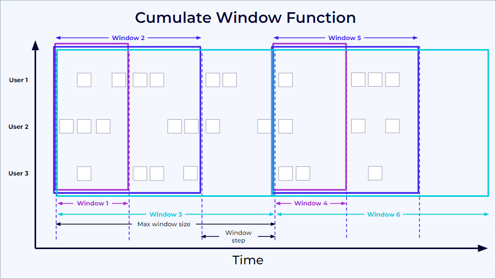
SinkUpsertMaterializer
When operating in upsert mode and processing two update events, a potential issue arises. If input operators for two tables in upsert mode are followed by a join and then a sink operator, update events might arrive at the sink out of order. If the downstream operator's implementation doesn't account for this out-of-order delivery, it can lead to incorrect results.
Flink typically determines the ordering of update history based on the primary key (or upsert keys) through a global analysis in the Flink planner. However, a mismatch can occur between the upsert keys of the join output and the primary key of the sink table. The SinkUpsertMaterializer operator addresses this mapping discrepancy.
This operator maintains a complete list of RowData in its state to correctly process any deletion events originating from the source table. However, this approach can lead to a significant state size, resulting in increased state access I/O overhead and reduced job throughput. Also the output value for each primary key is always the last (tail) element in the maintained list. It is generally advisable to avoid using SinkUpsertMaterializer whenever possible.
Consider a scenario where 1 million records need to be processed across a small set of 1,000 keys. In this case, SinkUpsertMaterializer would need to store a potentially long list, averaging approximately 1,000 records per key.
To mitigate the usage of SinkUpsertMaterializer:
- Ensure that the partition keys used for deduplication, group aggregation, etc., are identical to the sink table's primary keys.
SinkUpsertMaterializeris unnecessary if retractions already use the same key as the sink primary key. When most rows are soon retracted, the materializer may retain far less state.- Utilize Time-To-Live (TTL) to limit the state size based on time.
- A higher number of distinct values per primary key directly increases the state size of the SinkUpsertMaterializer.
Row pattern recognition
Find the longest period of time for which the average price of a stock did not go below a value
Create a Datagen to publish StockTicker to a Kafka topic. See product documentation on CEP pattern with SQL
create table StockTicker(symbol string, price int, tax int) with ('connector' = 'kafka',...)
SELECT * FROM StockTicker
MATCH_RECOGNIZE (
    partition by symbol
    order by rowtime
    measures
        FIRST(A.rowtime) as start_tstamp,
        LAST(A.rowtime) as last_tstamp,
        AVG(A.price) as avgPrice
    ONE ROW PER MATCH
    AFTER MATCH SKIP PAST LAST ROW
    PATTERN (A+ B)
    DEFINE
        A as AVG(A.price) < 15
);
MATCH_RECOGNIZE helps to logically partition and order the data that is used with the PARTITION BY and ORDER BY clauses, then defines patterns of rows to seek using the PATTERN clause. The logical components of the row pattern variables are specified in the DEFINE clause. B is defined implicitly as not being A.
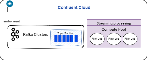
Confluent Cloud Specifics
See Flink Confluent Cloud queries documentation.
Each topic maps to a table with metadata columns such as $rowtime, aligned to the Kafka record timestamp. To inspect columns and watermarks, run DESCRIBE EXTENDED table_name;. With watermarking, arriving events are processed roughly in order with respect to $rowtime.
Mapping from Kafka record timestamp and table $rowtime
The Kafka record timestamp maps to $rowtime, a read-only field. Use it to order rows by ingestion time:
How to run Confluent Cloud for Flink?
See the note, but can be summarized as: 1/ create a stream processing compute pool in the same environment and region as the Kafka cluster, 2/ use Console or CLI (flink shell) to interact with topics.
Running Confluent Cloud Kafka with local Flink
The goal is to show how to use a Confluent Cloud cluster and send messages via Flink Faker from a local table into a Kafka topic:
See the scripts and README.
Here is an example of Faker definition for Confluent Cloud:
CREATE TABLE `rides` (
    `ride_id` STRING,
    `driver_id` STRING,
    `pickup_location` STRING,
    `dropoff_location` STRING,
    `pickup_time` TIMESTAMP(3),
    `dropoff_time` TIMESTAMP(3),
    `distance` DOUBLE,
    `fare` DOUBLE,
    `payment_type` STRING,
    `rating` DOUBLE
) WITH (
    'connector' = 'faker',
    'rows-per-second' = '4',
    'fields.ride_id.expression' = '#{Internet.UUID}',
    'fields.driver_id.expression' = '#{numerify ''driver_##''}',
    'fields.pickup_location.expression' = '#{Address.city}',
    'fields.dropoff_location.expression' = '#{Address.city}',
    'fields.pickup_time.expression' = '#{date.past ''5'',''1'',''SECONDS''}',
    'fields.dropoff_time.expression' = '#{date.past ''5'',''1'',''SECONDS''}',
    'fields.distance.expression' = '#{number.numberBetween ''10'',''100''}',
    'fields.fare.expression' = '#{number.numberBetween ''10'',''130''}',
    'fields.payment_type.expression' = '#{Options.option ''credit_card'', ''debit_card'', ''cash''}',
    'fields.rating.expression' = '#{number.numberBetween ''1'',''5''}'
    );
Reading from a topic at specific offsets
Create a long-running SQL job with the CLI
Get or create a service account.
Analyzing Statements
Assess the current Flink statement running in Confluent Cloud
To see which jobs are running, failed, or stopped, use the Confluent Cloud UI (Flink workspace) or the confluent CLI:
Understand the physical execution plan for a SQL query
See the EXPLAIN statement or Confluent Flink documentation for how to read the plan.
Indentation indicates data flow, with each operator passing results to its parent.
Review the state size, the changelog mode, the upsert key... Operators change changelog modes when different update patterns are needed, such as when moving from streaming reads to aggregations.
Pay special attention to data skew when designing your queries. If a particular key value appears much more frequently than others, it can lead to uneven processing where a single parallel instance becomes overwhelmed handling that key’s data. Consider strategies like adding additional dimensions to your keys or pre-aggregating hot keys to distribute the workload more evenly. Whenever possible, configure the primary key to be identical to the upsert key.
Troubleshooting SQL statement running slow
How to search for hot key?
A more advanced statistical query ( TO BE TESTED)
WITH key_stats AS (
    SELECT
        id,
        tenant_id,
        count(*) as record_count
    FROM src_aqem_tag_tag
    GROUP BY id, tenant_id
),
distribution_stats AS (
    SELECT
        AVG(record_count) as mean_count,
        STDDEV(record_count) as stddev_count,
        PERCENTILE_APPROX(record_count, 0.75) as q3,
        PERCENTILE_APPROX(record_count, 0.95) as p95,
        PERCENTILE_APPROX(record_count, 0.99) as p99
    FROM key_stats
)
SELECT
    ks.*,
    ds.mean_count,
    ds.stddev_count,
    -- Z-score calculation for outlier detection
    CASE
        WHEN ds.stddev_count > 0
        THEN (ks.record_count - ds.mean_count) / ds.stddev_count
        ELSE 0
    END as z_score,
    -- Hot key classification
    CASE
        WHEN ks.record_count > ds.p99 THEN 'EXTREME_HOT'
        WHEN ks.record_count > ds.p95 THEN 'VERY_HOT'
        WHEN ks.record_count > ds.q3 * 1.5 THEN 'HOT'
        ELSE 'NORMAL'
    END as hot_key_category
FROM key_stats ks
CROSS JOIN distribution_stats ds
WHERE ks.record_count > ds.mean_count
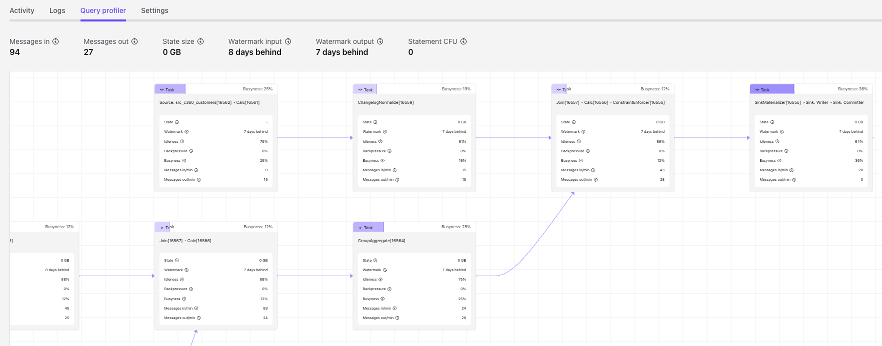
Confluent Flink Query Profiler
This is a Confluent-specific view of Flink performance, related to the Flink Web UI, for monitoring statement execution.