Deep learning
Update
Created 2021 - Updated 1/2026
Deep learning is a machine learning techniques which uses neural networks with more than one layer.
Neural Network
A Neural Network is a programming approach, based on the biological inspired neuron, used to teach a computer from training data instead of programming it with structured code.
The basic structure of a neural network includes an input layer (called "feature vector"), where the data is fed into the model, hidden layers that perform the computational processing, and an output layer that generates the final result. (See YouTube video: "Neural Network the ground up").
A classical learning example of neural network usage, is to classify images, like the hand written digits of the NIST dataset (shallow_net_demo.ipynb). For deeper networks, see Deep_net_keras.ipynb and intermediate_nn_keras_demo.ipynb.
A simple neuron holds a function that returns a number between 0 and 1. For example in simple image classification, neuron may hold the grey value of a pixel of a 28x28 pixels image (784 neurons). The number is called activation. At the output layer, the number in the neuron represents the percent of one output being the expected response. Neurons are connected together and each connection is weighted.
Convolutional neural networks (CNNs) (lenet_in_keras.ipynb) allows input size to change without retraining. For the grey digit classification, the CNN defines a neuron as a unique image pattern of 3x3. The output of the regression neural network is numeric, and the classification output is a class.
The value of the neuron 'j' in the next layer is computed by the classical logistic equation taking into account previous layer neurons (a) (from 1 to n (i being the index on the number of input)) and the weight of the connection (a(i) to neuron(j)):
To get the activation between 0 and 1, it uses the sigmoid function, the bias is a number to define when the neuron should be active.
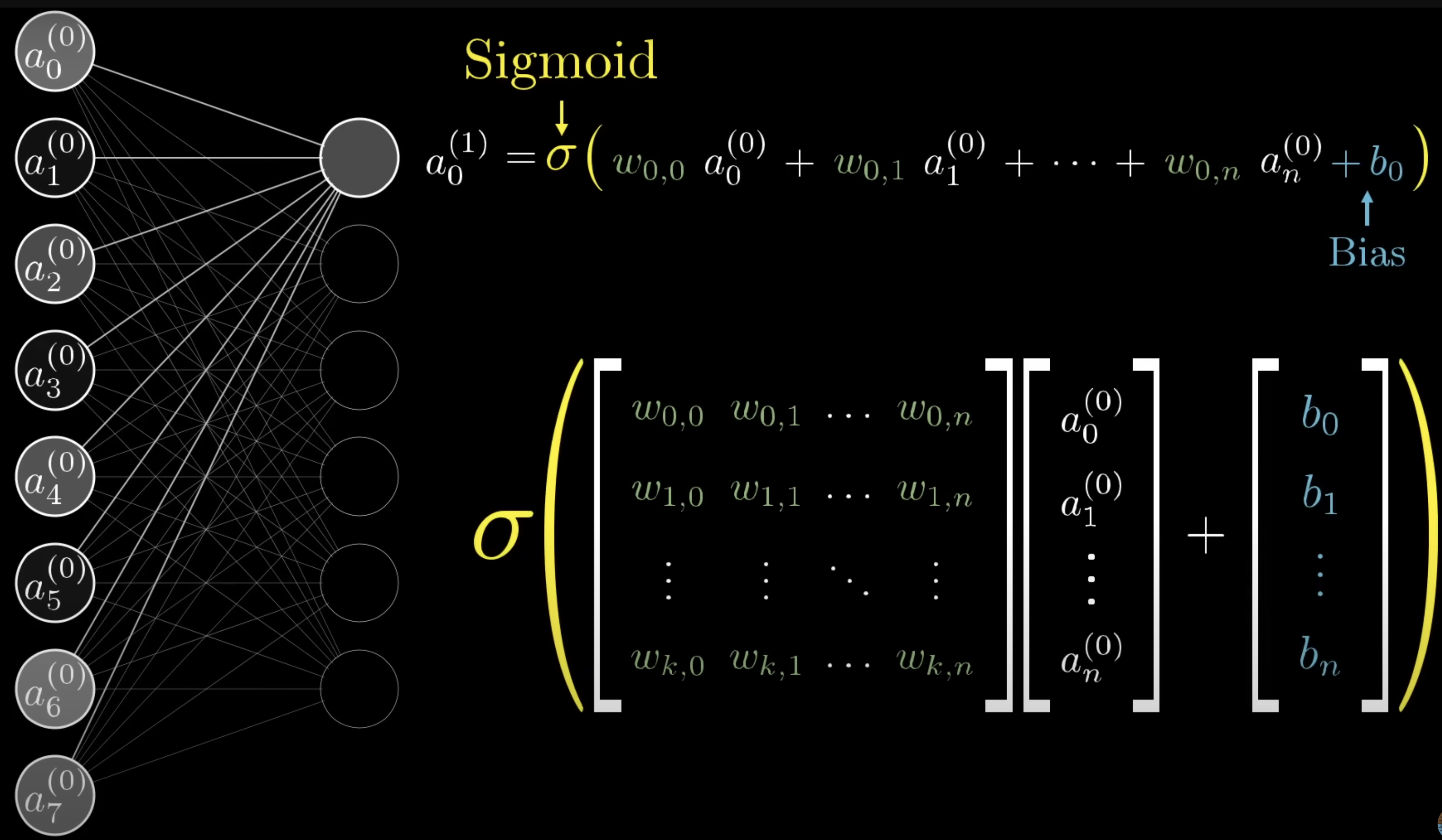
Modern neural network does not use sigmoid function anymore but the Rectifier Linear unit function.
Neural networks input and output can be an image, a series of numbers that could represent text, audio, or a time series...
The simplest architecture is the perceptron, represented by the following diagram:
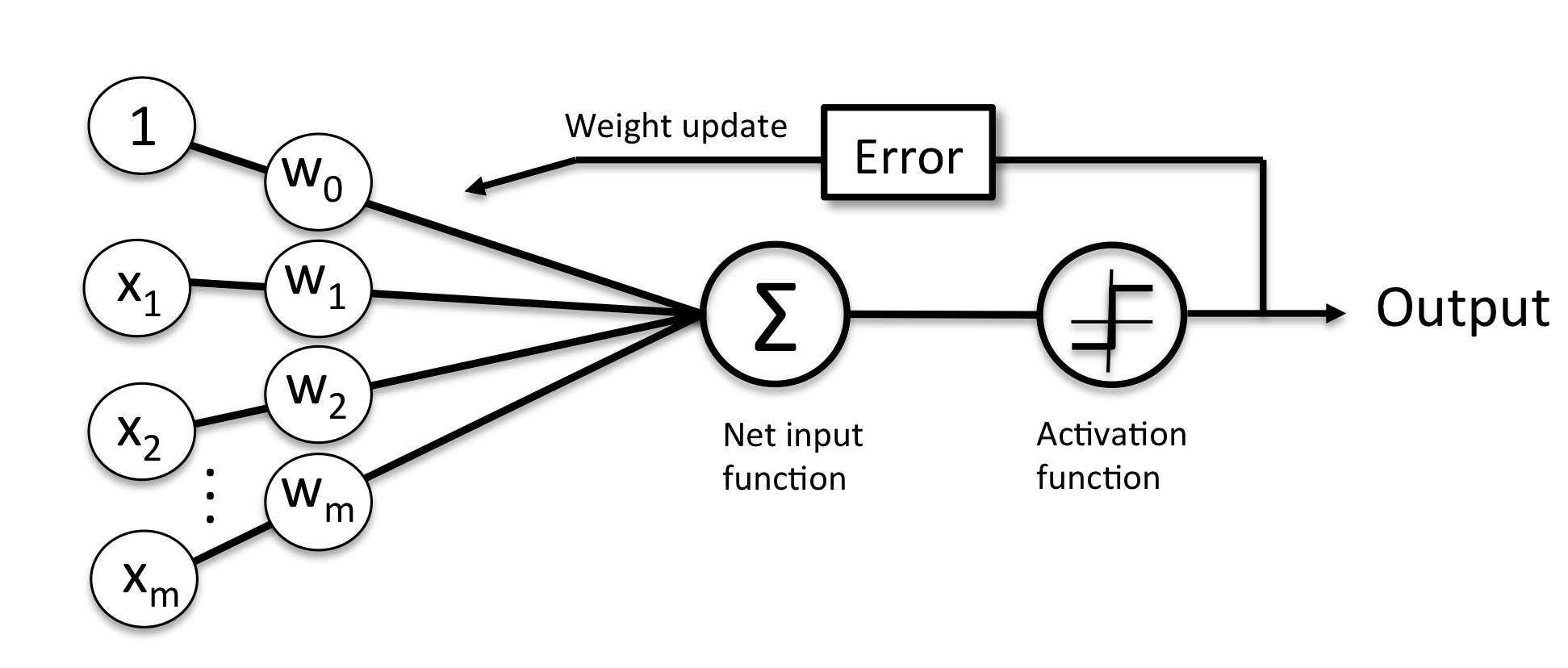
There are four types of neurons in a neural network:
- Input Neurons - We map each input neuron to one element in the feature vector.
- Hidden Neurons - Hidden neurons allow the neural network to be abstract and process the input into the output. Each layer receives all the output of previous layer.
- Output Neurons - Each output neuron calculates one part of the output.
- Bias Neurons - Work similar to the y-intercept of a linear equation. It introduces a 1 as input.
Neurons is also named nodes, units or summations. See the sigmoid play notebook to understand the effect of bias and weights
Training refers to the process that determines good weight values.
It is possible to use different Activation functions,(or transfer functions), such as hyperbolic tangent, sigmoid/logistic, linear activation function, Rectified Linear Unit (ReLU), Softmax (used for the output of classification neural networks), Linear (used for the output of regression neural networks (or 2-class classification)).
ReLU activation function is popular in deep learning because the gradiant descend function needs to take the derivative of the activation function. With sigmoid function, the derivative quickly saturates to zero as it moves from zero, which is not the case for ReLU.
The two most used Python frameworks for deep learning are TensorFlow/Keras (Google) or PyTorch (Facebook).
For hands-on introduction to these frameworks, see:
- Keras.ipynb - Keras basics with MNIST classification
- Tensorflow.ipynb - TensorFlow 2.x introduction
- torch-tensor-basic.ipynb - PyTorch tensor operations
- workflow-basic.ipynb - PyTorch ML workflow
Classification neural network architecture
The general architecture of a classification neural network.
| Hyperparameter | Classification |
|---|---|
| Input layer shape (in_features) | Same as number of features |
| Hidden layer(s) | Problem specific, minimum = 1, maximum = unlimited |
| Neurons per hidden layer | Problem specific, generally 10 to 512 |
| Output layer shape (out_features) | for binary 1 class, for multi-class: 1 per class |
| Hidden layer activation | Usually ReLU but can be many others |
| Output activation | For binary: Sigmoid, for multi-class: Softmax |
| Loss function | Binary cross entropy. For multi-class Cross entropy |
| Optimizer | SGD (stochastic gradient descent), Adam (see torch.optim for more options) |
Below is an example of a very simple NN in PyTorch, without any activation function:
from torch import nn

model_0 = nn.Sequential(
    nn.Linear(in_features=2, out_features=5),  # layer 1
    nn.Linear(in_features=5, out_features=1)   # layer 2
).to(device)

model_0
We can use a subclass of pyTorch nn.Module to define the NN. See demonstration in classifications.ipynb notebook, to search for the circle classes in the sklearn circles dataset, or a multi classes classification in multiclass-classifier.ipynb.
Recurrent Neural Networks (RNN)
Recurrent Neural Networks are designed to process sequential data where the order of inputs matters. Unlike feedforward networks, RNNs maintain a hidden state that captures information about previous inputs in the sequence.
Long Short-Term Memory (LSTM)
Standard RNNs suffer from the vanishing gradient problem, making it difficult to learn long-range dependencies. LSTM networks address this with a gating mechanism that controls information flow:
- Forget gate: decides what information to discard from the cell state
- Input gate: decides which values to update
- Output gate: decides what to output based on the cell state
from tensorflow.keras.layers import LSTM, Dense, Embedding
from tensorflow.keras.models import Sequential

model = Sequential([
    Embedding(vocab_size, embedding_dim, input_length=max_length),
    LSTM(128, return_sequences=True),
    LSTM(64),
    Dense(1, activation='sigmoid')
])
Use Cases
- Sentiment analysis: classifying text as positive/negative based on word sequences
- Time series prediction: forecasting stock prices, weather, sensor data
- Language modeling: predicting the next word in a sequence
- Speech recognition: converting audio sequences to text
See the Keras-RNN.ipynb notebook for a sentiment analysis example using LSTM on movie reviews from the IMDB dataset.
Learning
Same as previous ML problems, we can use supervised ( picture and corresponding classes) and unsupervised learning. For image or voice, the 'self-supervised learning' uses to generate supervisory signals for training data sets by looking at the relationships in the input data.
Transfer learning combine a first neural network as input to a second NN.
GPU vs CPU
- When the training loss is way lower than the test loss, it means "overfitting" and so loosing time.
- When both losses are identical, time will be wasted if we try to regularize the model.
- To optimize deep learning we need to maximize the compute-bound processing by reducing time spent on memory transfer and other things. Bandwidth cost is by moving the data from CPU to GPU, from one node to another, or even from CUDA global memory to CUDA shared memory.
Regularization Techniques
Regularization helps prevent overfitting by adding constraints to the model during training.
L1 Regularization (Lasso): Adds the absolute value of weights to the loss function. Produces sparse models by driving some weights to zero.
L2 Regularization (Ridge/Weight Decay): Adds the squared magnitude of weights to the loss function. Penalizes large weights without forcing them to zero.
In PyTorch, L2 regularization is implemented via the weight_decay parameter in optimizers:
Dropout: Randomly sets a fraction of input units to zero during training, which prevents neurons from co-adapting. Typical dropout rates are 0.2-0.5.
Batch Normalization: Normalizes layer inputs to have zero mean and unit variance. This stabilizes training, allows higher learning rates, and provides slight regularization.
Data Augmentation
Data augmentation artificially increases training set diversity by applying random transformations to input data. This improves model generalization without collecting more data.
For image data, torchvision.transforms provides common augmentations:
from torchvision import transforms

train_transform = transforms.Compose([
    transforms.Resize((224, 224)),
    transforms.RandomHorizontalFlip(p=0.5),
    transforms.RandomRotation(degrees=15),
    transforms.ColorJitter(brightness=0.2, contrast=0.2),
    transforms.ToTensor(),
    transforms.Normalize(mean=[0.485, 0.456, 0.406], std=[0.229, 0.224, 0.225])
])
Research shows that random transforms like TrivialAugmentWide and RandAugment generally outperform hand-picked transforms:
from torchvision.transforms import v2
train_transform = v2.Compose([
    v2.Resize((224, 224)),
    v2.TrivialAugmentWide(num_magnitude_bins=31),
    v2.ToTensor()
])
Data augmentation is applied only to training data, not validation or test sets.
Computer Image
Address how a computer sees, images.
Convolutional Neural Network
A Neural Network to process images by assigning learnable weights and biases to various aspects/objects in the image, and be able to differentiate one from the other. It can successfully capture the spatial and temporal dependencies in an image through the application of relevant filters.
Image has three matrices of values matching the size of the picture (H*W) and the RGB value R matrix, G and B matrices. CNN reduces the size of the matrices without loosing the meaning. For that, it uses the concept of Kernel, a window, shifting over the image.
A typical structure of a convolutional neural network:
Input layer -> [Convolutional layer -> activation layer -> pooling layer] -> Output layer
The layers between [] can be replicated.
Every layer in a neural network is trying to compress data from higher dimensional space to lower dimensional space. Below is an example of this method:
# Convolutional layer
nn.Conv2d(in_channels=input_shape, out_channels=hidden_units, kernel_size=3, stride=1, padding=1),
nn.ReLU(),  # activation layer
# pooling layer
nn.MaxPool2d(kernel_size=2, stride=2),
- Conv2d is compressing the information stored in the image to a smaller dimension image
- MaxPool2d takes the maximum value from a portion of a tensor and disregard the rest.
See this CNN explainer tool.
Simple image dataset using the Fashion NIST.
Code examples for CNN implementations:
- fashion_cnn.py - PyTorch CNN for Fashion MNIST
- tiny_vgg.py - TinyVGG architecture implementation
- computer_vision.ipynb - Computer vision notebook walkthrough
- Keras-CNN.ipynb - CNN with Keras for MNIST digit classification
- AlexnetJb.ipynb - AlexNet implementation
MIT - Convolutional Neural Network presentation - video
Transfer Learning
Take an existing pre-trained model, and use it on our own data to fine tune the parameters. It helps to get better results with less data, and lesser cost and time. In Computer Vision, Image Net includes million of images on which models were trained.
PyTorch has pre-trained models, Hugging Face too, PyTorch Image Models - Timm is a collection of image models, layers, utilities, optimizers, schedulers, data-loaders / augmentations, and reference training / validation scripts that can be reused. Paper with code is a collection of the latest state-of-the-art machine learning papers with code implementations attached to the article.
The custom data going into the model needs to be prepared in the same way as the original training data that went into the model:
# load existing NN weights
weights = torchvision.models.EfficientNet_B0_Weights.DEFAULT
# Get the transforms used to create our pretrained weights
transformer= weights.transforms()
The transformer is used to create the data loaders:
train_dl,test_dl, classes=data_setup.create_data_loaders(
                            train_dir,
                            test_dir,
                            transformer,
                            transformer,
                            batch_size=BATCH_SIZE)
Then, take an existing model. Often bigger models are better but results may also being linked to the type of device used and the hardware resource capacity. efficientnet_b0 has 288,548 parameters.
efficientnet_b0 parts
efficientnet_b0 comes in three main parts:
- features: A collection of convolutional layers and other various activation layers to learn a base representation of vision data.
- avgpool: Takes the average of the output of the features layer(s) and turns it into a feature vector.
- classifier: Turns the feature vector into a vector with the same dimensionality as the number of required output classes (since efficientnet_b0 is pretrained on ImageNet with 1000 classes.
The process of transfer learning usually goes: freeze some base layers of a pre-trained model (typically the features section) and then adjust the output layers (also called head/classifier layers) to suit the needs.
for param in model.features.parameters():  # Freeze the features
    param.requires_grad = False

model.classifier = torch.nn.Sequential(
        torch.nn.Dropout(p=0.2, inplace=True),
        torch.nn.Linear(in_features=1280,
                        out_features=len(classes),
                        bias=True)).to(device)
Dropout layers randomly remove connections between two neural network layers with a probability of p. This practice is meant to help regularize (prevent overfitting) a model by making sure the connections that remain learn features to compensate for the removal of the other connections.
See PyTorch transfer learning for image classification code.
Distributed Training
Training large models requires distributing computation across multiple GPUs or machines. PyTorch provides Distributed Data Parallel (DDP) for this purpose.
DDP replicates the model across GPUs, splits data batches, and synchronizes gradients after each backward pass using the Ring AllReduce algorithm. This allows training to scale efficiently while maintaining model consistency.
from torch.nn.parallel import DistributedDataParallel as DDP
from torch.distributed import init_process_group

# Setup process group
init_process_group(backend="nccl", rank=rank, world_size=world_size)

# Wrap model with DDP
model = DDP(model, device_ids=[gpu_id])
For multi-GPU training with fault tolerance, use torchrun:
See the Distributed Data Parallel documentation for detailed coverage and the following code examples:
- multi_gpu_ddp.py - Basic DDP implementation
- multi_gpu_torchrun.py - Training with torchrun
- multinode.py - Multi-machine training
Practical Projects
For a hands-on project applying deep learning concepts, see DeepLearningProject-Solution.ipynb which builds a Multi-Layer Perceptron to classify mammogram masses as benign or malignant.
Sources of information
- HuggingFace deep reinforcement
- Dive into Deep Learning - Comprehensive online book from Amazon
- Learn PyTorch for deep learning - Zero to mastery course
- Horace He - Making Deep Learning Go Brrrr From First Principles
- MIT - Convolutional Neural Network presentation - video
- Jeff Heaton - Applications of Deep Neural Networks - WashU course materials
- PyTorch documentation
- TensorFlow/Keras documentation
- Papers with Code - State-of-the-art papers with implementations